Take \(d\) independent tosses of a biased coin, which lands heads with probability \(c/d\), for constant \(c \le 0.5d\). Now, you count the number of heads you observe, and if this number is odd, you write down "head", and otherwise, you write down "tail". Surprisingly, you can obtain an almost fair coin this way.
Equivalently, let’s observe a sequence of bits \(\textbf{x} = x_1x_2...x_d\). Each bit \(x_i\) is 1 with probability \(c/d, c \le 0.5d\) and is 0 otherwise. Then the parity of this sequence has only exponential bias. Concretely,
\[\mathbb{P}[\chi(\textbf{x})= 1] = \frac{1}{2} \pm \exp(\Omega(c))\]
where \(\chi\) is the parity function, i.e. \(\chi(\textbf{x}) =\sum_i x_i \text{ mod } 2\).
This claim turns out to be extremely easy to show after a basic introduction to finite, irreducible, ergodic Markov chains.
Crash Course: Markov Chains
Let \(S\) be a finite state space and \(T\) denote time which is a subset of \(\mathbb{N}\cup\{0\}\). A stochastic process is a sequence of random variables \(\{X_n: n \in T\}\) which take values from \(S\). If \(X_n = i\), we say that the process is in state \(i\) at time
\(n\). Suppose that \[\mathbb{P}[X_{n + 1} = j | X_n = i, X_{n - 1} = i_{n - 1}, ..., X_1 = i_1, X_0 = i_0] = \mathbb{P}[X_{n + 1} = j | X_n = i] = p_{i,j}\] for all states \(i_0, i_1, ..., i, j \in S\) and all \(n \ge 0\). Then this sequence of conditional probabilities is also a sequence of random variables, and this stochastic process is known as a finite Markov chain. Informally, this states that the future is independent of the past given the present.
The transition matrix \(\textbf{P}= (p_{i,j})\) is a \(|S| \times |S|\) matrix of transition probabilities, where
\(p_{i,j} = \mathbb{P}(X_{n+1} = j|X_n = i)\). \[\textbf{P} = \begin{bmatrix} p_{00} & p_{01} & p_{02} & \cdots \\ p_{10} & p_{11} & p_{12} & \cdots \\ \vdots & \vdots & \vdots & \\ p_{i0} & p_{i1} & p_{i2} & \cdots \\ \vdots & \vdots & \vdots & \\ \end{bmatrix}\]
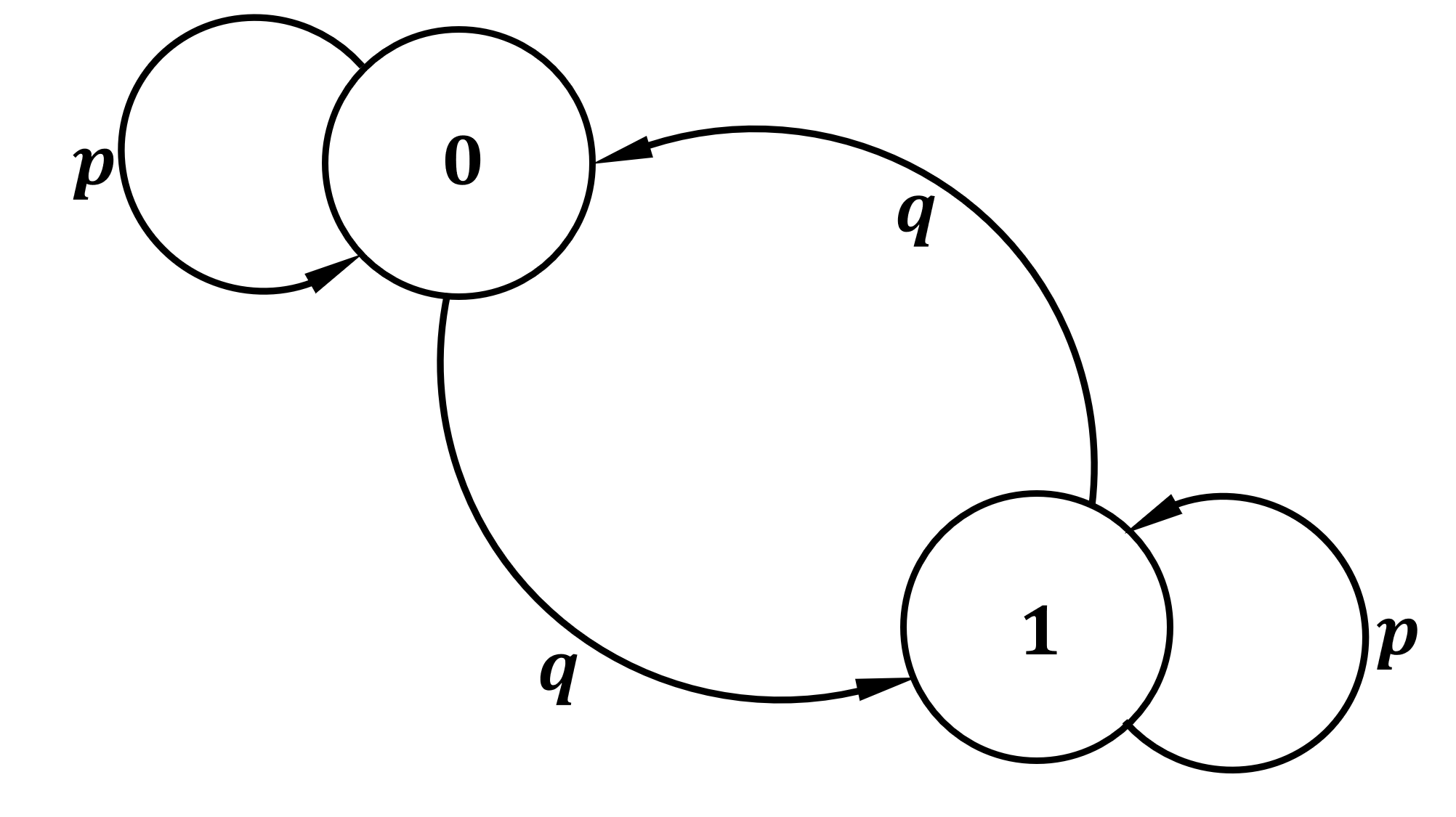
In our example, we have two states: \(0\) (an even number of heads after \(d\) flips) and \(1\) (an odd number of heads). Let us define our transition probabilities to be \(p = 1 - c/d\) (the probability of flipping tails), and \(q = c/d\) (the probability of heads). If this chain is in state \(0\) during time \(n\), i.e. \(X_n = 0\), then the process will remain in state \(0\) with probability \(p_{0,0} = p\) and transition to state \(1\) with probability \(p_{0,1} = q\). Similarly, if \(X_n = 1\), then \(p_{1,0} = q\), and \(p_{1,1} = p\). Thus, we obtain our transition matrix \[\textbf{Q} = \begin{bmatrix} p & q \\ q & p \\ \end{bmatrix}\]
We say that a finite Markov chain is irreducible if and only if its graph representation is a strongly connected graph. That is, each state (represented by a vertex/node) is reachable from all of the other states with non-zero probability. As can be seen in the graph representation of \(\textbf{Q}\) below, \(\textbf{Q}\) is irreducible.
Periodicity
Let \(\textbf{Q}(n)\) be the transition matrix at time \(n\), and \(p_{i,j}(n)\) be the \(ij\)-th entry of this matrix. Then, the period of a state \(i\) is the greatest common divisor of the set \(\{n: p_{i,i}(n) > 0, n\ge 1\}\), i.e. the set of times in which state \(i\) is reachable. We write \(d(i) = \gcd\{n: p_{i,i}(n) > 0, n\ge 1\}\). Thus, for a chain whose current state is \(i\), it is impossible for the chain to return to state \(i\) in \(t\) steps unless \(t\) is divisible by \(d(i)\).
We call state \(i\) periodic if \(d(i) > 1\) and aperiodic if \(d(i) = 1\). We notice that in our transition matrix \(\textbf{Q}\), \(p_{i,i} > 0\) for \(i = 0,1\). This means that in each step, we can get back to the last state with positive probability; therefore, our Markov chain is aperiodic.
Recurrence
Let \(f_{i,i}(n) = \mathbb{P}[X_n = i, X_k \ne i \text{ for } 0 < k < n | X_0 = i]\); that is, \(f_{i,i}(n)\) is the probability that the chain will return to its beginning state for the first time at time \(n\). Next, let \(f_{i,i}\) be the probability that given \(X_0 = i\), \(X_n = i\) for some \(n > 0\). That is, \[f_{i,i} = \sum_{n = 1}^{\infty}f_{i,i}(n)\] State \(i\) is said to be recurrent if \(f_{i,i} = 1\). Informally, if a chain’s beginning state \(i\) is recurrent, then the chain will eventually return to state \(i\) with probability 1. Alternatively, we say that state \(i\) is transient if \(f_{i,i} < 1\).
For a recurrent state, the mean recurrence time \(\mu_i\) is defined as: \[\mu_i = \sum_{n=1}^\infty nf_{i,i}(n)\]
The mean recurrence time is the expected amount of time for the chain to return to its beginning state.
A recurrent state \(i\) is called positive recurrent if \(\mu_i < \infty\). Notice that a recurrent state \(i\) can have infinite mean recurrence time. Such a state is called null recurrent. A state is said to be ergodic if it is positive recurrent and aperiodic. A Markov chain is ergodic if all states are ergodic.
In our example, given that the chain is in state \(0\), in the next coin flip, the chain either remains in state \(0\) with probability \(p\) (flipping a tail), or transitions to state \(1\) with probability \(q\) (flipping a head). Alternatively, if the chain is in state \(1\), then in the next coin flip, the chain remains in state \(1\) with probability \(p\), or transitions to state \(0\) with probability \(q\). Therefore, the mean recurrence times for our chain are: \[\mu_0 = \sum_{k} nf_{0,0}(k) = p + q\sum_{k = 0}^{\infty}(k+1)p^kq\] And: \[\mu_1 = \sum_{k} nf_{1,1}(k) = p + q\sum_{k = 0}^{\infty}(k+1)p^kq\] Notice that \(\sum_{k = 0}^{\infty}kp^kq\) is the expectation of a geometric distribution with probability \(q\) and \(\sum_{k = 0}^{\infty}p^kq\) is the sum of the probability mass of the same geometric distribution. Thus, as \(\sum_{k = 0}^{\infty}(k+1)p^kq = \sum_{k = 0}^{\infty}kp^kq + \sum_{k = 0}^{\infty}p^kq = 1/q + 1\), \[\mu_0 = \mu_1 = p + q\cdot (1/q + 1) = 2\] Hence, both states of our Markov chain are positive recurrent. In fact, this Markov chain is ergodic.
Stationary distributions
A stationary distribution of a Markov chain is a probability distribution \(\bar \pi\) such that \(\bar \pi \textbf{P} = \bar \pi\). In other words, \(\bar{\pi}\) is the long-term limiting distribution of the chain. In fact, any finite, irreducible, and ergodic Markov chain has a unique stationary distribution \(\bar \pi =(\pi_0,\pi_1,...,\pi_n)\), with \(\pi_0 + \pi_1 + ... + \pi_n = 1\) (Theorem 7.7 in Mitzenmacher and Upfal (2017)). Hence, for our example:
\[\bar \pi \textbf{Q} = [\pi_0, \pi_1] \begin{bmatrix} p & q \\ q & p \\ \end{bmatrix} = \bar \pi\hspace{2cm}\pi_0 + \pi_1 = 1\] This produces a system of equations whose solution gives us that \(\pi_0 = \pi_1 = 1/2\). This tells us that if you flip a biased coin an infinite number of times, you can place a bet on the parity of the number of heads and win half of the time. In other words, \[\mathbb{P}[\chi(x_1x_2...) = 1] = 1/2\]
How fast does the probability converge to \(1/2\) with respect to the number of coin tosses? In fact, this convergence is geometric.
Now we are ready to prove the bound for our motivating example. Since \(c \le 0.5d\), we have \(q < p\). Thus, if we take \(d\) coin tosses, \[|| \bar\pi^n_0 - \bar\pi || \le (1- 2q)^d = (1 - 2\cdot \frac{c}{d})^d \le \exp(-2c)\]
In summary, the probability of obtaining an odd number of heads is within \(\pm \exp(-2c)\) of \(0.5\).
For a fixed value of \(c\) and \(d\), the probability distribution for \(X_d\) can be computed exactly. First, define the initial distribution to be \(\pi = \left[\mathbb{P}(X_0 = 0), \mathbb{P}(X_0 = 1)\right] = [1,0]\). Then, \(X_d\) has distribution \(\pi\cdot\textbf{Q} = \pi \cdot\begin{bmatrix}p & q \\q & p \end{bmatrix}^d\). Thus, for \(c = 1, d = 10\), the distribution of \(X_{10}\) is \([\mathbb{P}(X_{10} = 0),\mathbb{P}(X_{10} = 1)] \approx [0.554, 0.446]\).
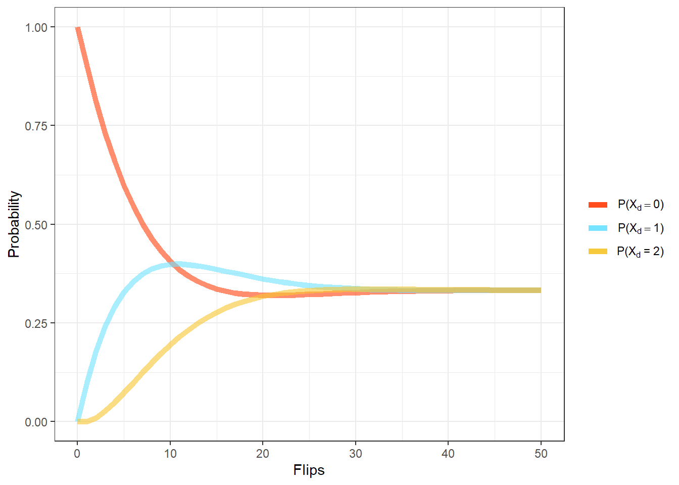
Fixing \(p= \frac 9 {10}\), the distribution of \(X_d\) can be studied for various values of \(d\).
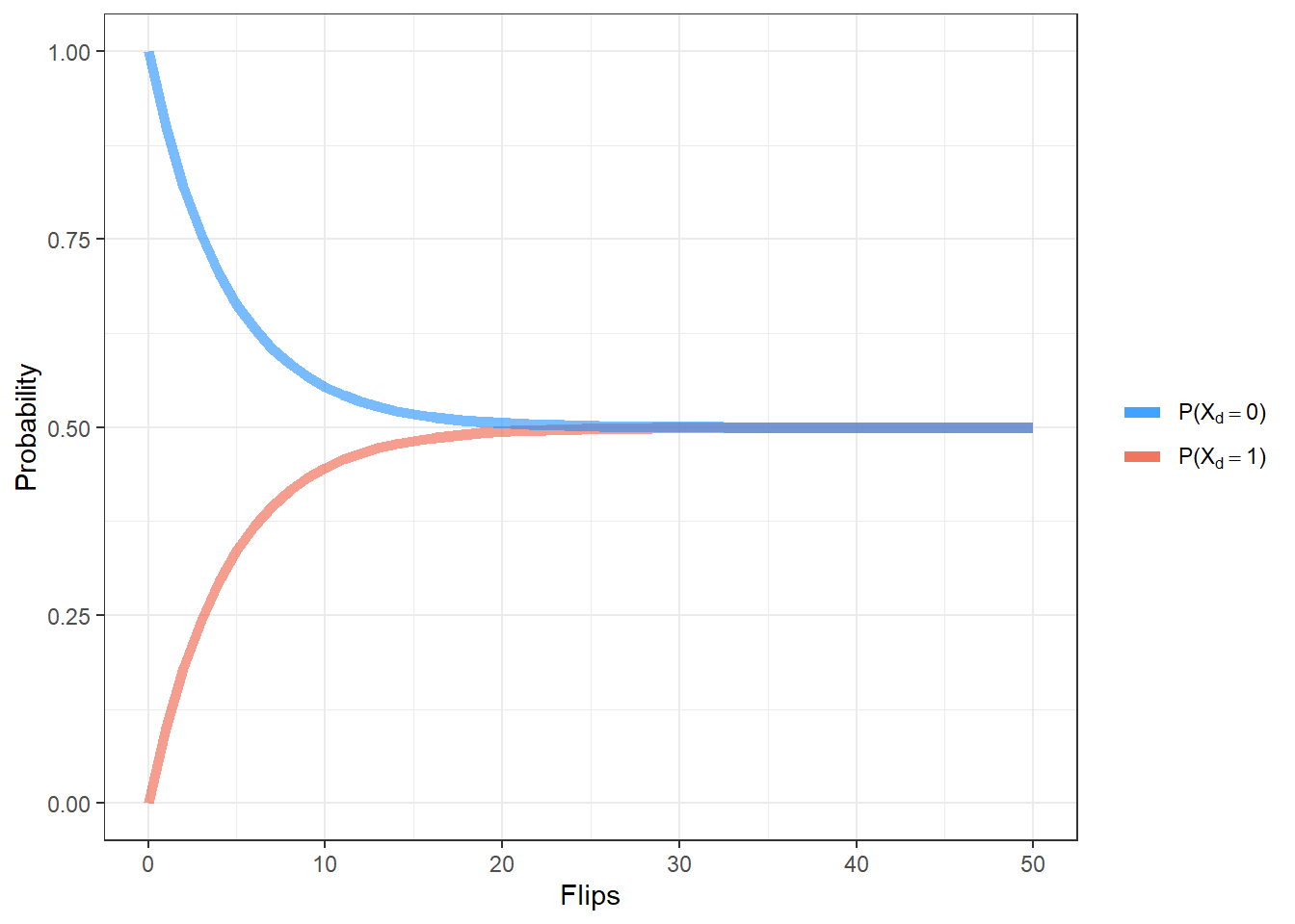
As to be expected, as \(d\) gets large, the probability that the number of heads will be odd converges to \(\frac 1 2\).
Generalization
Modulo \(m\)
What happens if we toss the same coin, but take modulo \(m\) in our final step instead of the parity? The transition matrix thus becomes \(m\times m\):
\[\textbf{Q} = \begin{bmatrix} p & q & 0 & 0 & ... & 0 & 0 \\ 0 & p & q & 0 & ... & 0 & 0 \\ \vdots & \vdots & \ddots & \ddots & \vdots & \vdots & \vdots\\ \vdots & \vdots & \vdots & \ddots & \ddots & \vdots & \vdots\\ \vdots & \vdots & \vdots & \vdots & \ddots & \ddots & \vdots\\ 0 & 0 & 0 & 0 & ... & p & q \\ q & 0 & 0 & 0 & ... & 0 & p \\ \end{bmatrix}\]
Notice that the graph of this Markov chain is exactly a cycle with self-loops. Again, \(\mu_i, i \in 0, ..., m-1\) are sums of geometric series, which are finite.
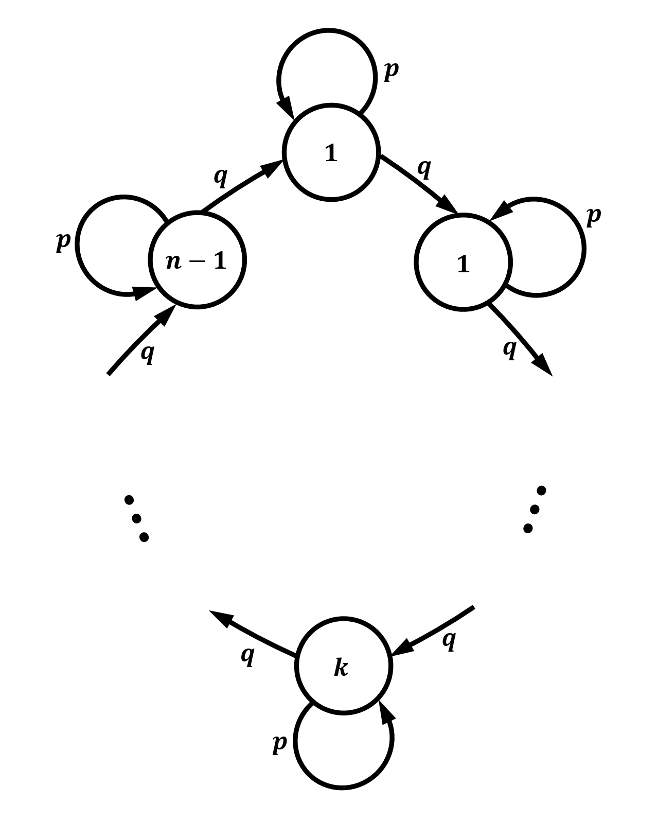
As for the stationary distribution, \[\bar \pi \textbf{Q} = (\pi_0, \pi_1, ... , \pi_{m-1}) = \bar \pi \hspace{2cm} \sum_{j = 0}^{m-1}\pi_j = 1\] gives us \(\pi_i = 1/n, i \in 0, ..., m-1\). That is, we obtain the uniform distribution as the number of flips goes to infinity. We cannot apply the coupling theorem directly because each of the columns of the transition matrix has 0’s.
In fact, we can see for a small value of \(d\), that the convergence to the uniform distribution is quite slow. For \(c = 1,d = 10\) and \(m = 3\), the distribution of \(X_d\) is far from uniform: \[[\mathbb{P}(X_{10} = 0),\mathbb{P}(X_{10} = 1),\mathbb{P}(X_{10} = 2)] = \pi\cdot\textbf{Q}^{10} =\begin{bmatrix}1& 0& 0\end{bmatrix}\cdot\begin{bmatrix}.9 & .1 & 0 \\0& .9 & .1 \\ .1 & 0 & .9\end{bmatrix}^{10} \approx \begin{bmatrix}0.406& 0.399& 0.195\end{bmatrix}\]
However, at around 30 tosses, the distribution approaches uniform.
\(m\)-sided dice
Let’s take this problem one step further. Suppose now we are instead tossing a \(m\)-sided die, which lands 0 with probability \(1 - c/d, c \le 0.5d\), and lands \(i\) with probability \(r = c/(d\cdot (m-1)), i = 1, ..., m-1\). Again, we take modulo \(m\) in our final step. In this case, the transition matrix becomes \[\textbf{Q} = \begin{bmatrix} p & r & ... & r & r \\ r & p & ... & r & r \\ \vdots & \vdots & \ddots & \vdots & \vdots \\ r & r & ... & p & r \\ r & r & ... & r & p \\ \end{bmatrix}\] which is a clique with self loops. The following lemma simplifies the verification of the positive recurrence of our example.
Without loss of generality, assume state \(0\) is positive recurrent. By symmetry, we obtain that this Markov chain is positive recurrent. The stationary distribution is again uniform, i.e. \(\pi_i = 1/n, i \in 0, ..., m-1\). The rate of convergence, however, is faster. \[|| \bar\pi^n_0 - \bar\pi || \le (1- mr)^d = (1 - m\cdot \frac{c}{d\cdot (m-1)})^d \le \exp(-c\cdot\frac{m}{m-1})\]
Fix \(c=1,d=10\). For a six sided die that rolls \(0\) with \(p=1-\frac c d = .9\), and rolls \(i\) with probability \(\frac{1-p}{5} = 0.02,i\in\{1,2,3,4,5\}\), then the distribution of \(X_{10}\) is: \[\pi\cdot\textbf{Q}^{10}=\begin{bmatrix}1&0&0&0&0&0\end{bmatrix}\cdot \begin{bmatrix}.9 & .02 & .02 & .02 & .02 & .02\\.02 & .9 & .02 & .02 & .02 & .02\\ .02 & .02 & .9 & .02 & .02 & .02\\.02 & .02 & .02 & .9 & .02 & .02\\.02 & .02 & .02 & .02 & .9 & .02\\.02 & .02 & .02 & .02 & .02 & .9\end{bmatrix}^{10} \approx \begin{bmatrix}0.399 & 0.12 & 0.12 & 0.12 & 0.12 & 0.12\end{bmatrix}\]
Fixing \(p\):
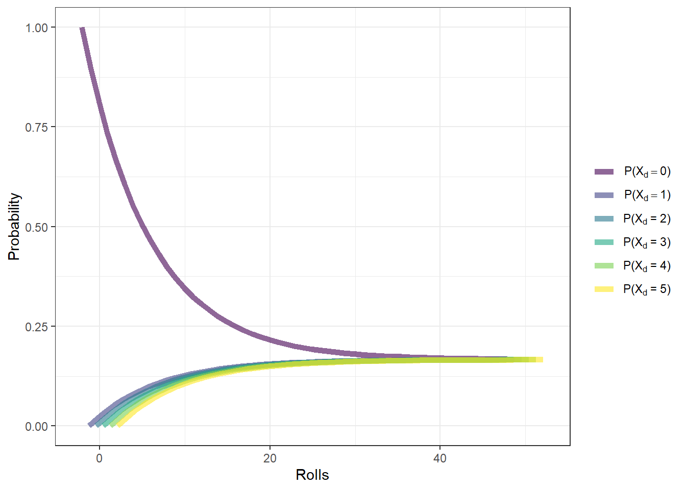
(A small amount of dodge has been added to help differentiate between the lines)
\(\blacksquare\)
Acknowledgements
We thank Dr. Joe Neeman for his insightful comments on earlier drafts.
References
Mitzenmacher, Michael, and Eli Upfal. 2017. Probability and Computing: Randomization and Probabilistic Techniques in Algorithms and Data Analysis. Cambridge university press.